

Kaggle Toxic Classification EDA
Introduction
-
Wikipedia에서 제공된 대량의 데이터 셋이 있고 이 중 clean한 comments와 toxcid 관련 comments가 섞여 있다. (사람이 라벨링) 이 중에서 toxic 관련 라벨 데이터는 6개 가지 라벨 종류로 되어 있고 한 comments에 대해 여러 라벨이 태깅될 수 있다. Test dataset에 대해 아래와 같은 라벨로 구분하는 모델을 만드는 것이 Toxic Classification 목적
-
Labels : toxic, severe_toxic, obscene, threat, insult, identity_hate
-
link : https://www.kaggle.com/c/jigsaw-toxic-comment-classification-challenge
Definition (Library & Functions)
#import required packages
#basics
import pandas as pd
import numpy as np

#misc
import gc
import time
import warnings

#stats
from scipy.misc import imread
from scipy import sparse
import scipy.stats as ss

#viz
import matplotlib.pyplot as plt
import matplotlib.gridspec as gridspec
import seaborn as sns
from wordcloud import WordCloud ,STOPWORDS
from PIL import Image
import matplotlib_venn as venn

#nlp
import string
import re    #for regex
import nltk
from nltk.corpus import stopwords
import spacy
from nltk import pos_tag
from nltk.stem.wordnet import WordNetLemmatizer
from nltk.tokenize import word_tokenize
# Tweet tokenizer does not split at apostophes which is what we want
from nltk.tokenize import TweetTokenizer


#FeatureEngineering
from sklearn.feature_extraction.text import TfidfVectorizer, CountVectorizer, HashingVectorizer
from sklearn.decomposition import TruncatedSVD
from sklearn.base import BaseEstimator, ClassifierMixin
from sklearn.utils.validation import check_X_y, check_is_fitted
from sklearn.linear_model import LogisticRegression
from sklearn import metrics
from sklearn.metrics import log_loss
from sklearn.model_selection import StratifiedKFold
from sklearn.model_selection import train_test_split


#settings
start_time=time.time()
color = sns.color_palette()
sns.set_style("dark")
eng_stopwords = set(stopwords.words("english"))
warnings.filterwarnings("ignore")

lem = WordNetLemmatizer()
tokenizer=TweetTokenizer()

%matplotlib inline
Function
highlighting the min and max value
# Using Pandas style API for highlighting the min and max for each stat
def highlight_min(s):
    '''
    highlight the minimum in a Series yellow.
    '''
    is_min = s == s.min()
    return ['background-color: red' if v else '' for v in is_min]

def highlight_max(s):
    '''
    highlight the maximum in a Series yellow.
    '''
    is_max = s == s.max()
    return ['background-color: green' if v else '' for v in is_max]
Function
define Cramer’s Correlation Stats
두 개의 categorical data에 대한 correlation을 파악할 때에는 cramers V가 optimistic한 방법 중 하나이다
#https://stackoverflow.com/questions/20892799/using-pandas-calculate-cram%C3%A9rs-coefficient-matrix/39266194
def cramers_corrected_stat(confusion_matrix):
    """ calculate Cramers V statistic for categorial-categorial association.
        uses correction from Bergsma and Wicher,
        Journal of the Korean Statistical Society 42 (2013): 323-328
    """
    chi2 = ss.chi2_contingency(confusion_matrix)[0]
    n = confusion_matrix.sum().sum()
    phi2 = chi2/n
    r,k = confusion_matrix.shape
    phi2corr = max(0, phi2 - ((k-1)*(r-1))/(n-1))
    rcorr = r - ((r-1)**2)/(n-1)
    kcorr = k - ((k-1)**2)/(n-1)
    return np.sqrt(phi2corr / min( (kcorr-1), (rcorr-1)))
Text 전처리
- 모두 소문자화, ip/user 형식 데이터 삭제, \n 삭제, aphostrophe replacement
def clean(comment):
    """
    This function receives comments and returns clean word-list
    """
    #Convert to lower case , so that Hi and hi are the same
    comment=comment.lower()
    #remove \n
    comment=re.sub("\\n","",comment)
    # remove leaky elements like ip,user
    comment=re.sub("\d{1,3}\.\d{1,3}\.\d{1,3}\.\d{1,3}","",comment)
    #removing usernames
    comment=re.sub("\[\[.*\]","",comment)

    #Split the sentences into words
    words=tokenizer.tokenize(comment)

    # (')aphostophe  replacement (ie)   you're --> you are
    # ( basic dictionary lookup : master dictionary present in a hidden block of code)
    words=[APPO[word] if word in APPO else word for word in words]
    words=[lem.lemmatize(word, "v") for word in words]
    words = [w for w in words if not w in eng_stopwords]

    clean_sent=" ".join(words)
    # remove any non alphanum,digit character
    #clean_sent=re.sub("\W+"," ",clean_sent)
    #clean_sent=re.sub("  "," ",clean_sent)
    return(clean_sent)
TF-IDF(Term Frequency - Inverse Document Frequency)
- 정보 검색과 텍스트 마이닝에서 이용하는 가중치로, 여러 문서로 이루어진 문서군이 있을 때 어떤 단어가 특정 문서 내에서 얼마나 중요한 것인지를 나타내는 통계적 수치
TF-IDF는 단어 빈도와 역문서 빈도의 곱
- 단어 빈도 tf(t,d)의 경우, 문서 내에 나타나는 해당 단어의 총 빈도수를 사용
- 역문서 빈도는 한 단어가 문서 집합 전체에서 얼마나 공통적으로 나타나는지를 나타내는 값
특정 문서 내에서 단어 빈도가 높을 수록, 그리고 전체 문서들 중 그 단어를 포함한 문서가 적을 수록 TF-IDF값이 높아짐 따라서 이 값을 이용하면 모든 문서에 흔하게 나타나는 단어를 걸러내는 효과를 얻을 수 있음
#https://buhrmann.github.io/tfidf-analysis.html
def top_tfidf_feats(row, features, top_n=25):
    ''' Get top n tfidf values in row and return them with their corresponding feature names.'''
    topn_ids = np.argsort(row)[::-1][:top_n]
    top_feats = [(features[i], row[i]) for i in topn_ids]
    df = pd.DataFrame(top_feats)
    df.columns = ['feature', 'tfidf']
    return df

def top_feats_in_doc(Xtr, features, row_id, top_n=25):
    ''' Top tfidf features in specific document (matrix row) '''
    row = np.squeeze(Xtr[row_id].toarray())
    return top_tfidf_feats(row, features, top_n)

def top_mean_feats(Xtr, features, grp_ids, min_tfidf=0.1, top_n=25):
    ''' Return the top n features that on average are most important amongst documents in rows
        indentified by indices in grp_ids. '''

    D = Xtr[grp_ids].toarray()

    D[D < min_tfidf] = 0
    tfidf_means = np.mean(D, axis=0)
    return top_tfidf_feats(tfidf_means, features, top_n)

# modified for multilabel milticlass
def top_feats_by_class(Xtr, features, min_tfidf=0.1, top_n=20):
    ''' Return a list of dfs, where each df holds top_n features and their mean tfidf value
        calculated across documents with the same class label. '''
    dfs = []
    cols=train_tags.columns
    for col in cols:
        ids = train_tags.index[train_tags[col]==1]
        feats_df = top_mean_feats(Xtr, features, ids, min_tfidf=min_tfidf, top_n=top_n)
        feats_df.label = label
        dfs.append(feats_df)
    return dfs
#Credis to AlexSanchez https://www.kaggle.com/jhoward/nb-svm-strong-linear-baseline-eda-0-052-lb#261316
#custom NB model

class NbSvmClassifier(BaseEstimator, ClassifierMixin):
    def __init__(self, C=1.0, dual=False, n_jobs=1):
        self.C = C
        self.dual = dual
        self.n_jobs = n_jobs

    def predict(self, x):
        # Verify that model has been fit
        check_is_fitted(self, ['_r', '_clf'])
        return self._clf.predict(x.multiply(self._r))

    def predict_proba(self, x):
        # Verify that model has been fit
        check_is_fitted(self, ['_r', '_clf'])
        return self._clf.predict_proba(x.multiply(self._r))

    def fit(self, x, y):
        # Check that X and y have correct shape
        y = y.values
        x, y = check_X_y(x, y, accept_sparse=True)

        def pr(x, y_i, y):
            p = x[y==y_i].sum(0)
            return (p+1) / ((y==y_i).sum()+1)

        self._r = sparse.csr_matrix(np.log(pr(x,1,y) / pr(x,0,y)))
        x_nb = x.multiply(self._r)
        self._clf = LogisticRegression(C=self.C, dual=self.dual, n_jobs=self.n_jobs).fit(x_nb, y)
        return self

# model = NbSvmClassifier(C=4, dual=True, n_jobs=-1)
wikipedia에서 제공하는 최근 날짜 기준으로 block된 IP list
blocked IP와 toxic comments는 관련이 높을 관련성이 많으므로 feature engineering 차원에서 하나의 idea로 pick할 수 있음
#https://en.wikipedia.org/wiki/Wikipedia:Database_reports/Indefinitely_blocked_IPs)

blocked_ips=["216.102.6.176",
"216.120.176.2",
"203.25.150.5",
"203.217.8.30",
"66.90.101.58",
"125.178.86.75",
"210.15.217.194",
"69.36.166.207",
"213.25.24.253",
"24.60.181.235",
"71.204.14.32",
"216.91.92.18",
"212.219.2.4",
"194.74.190.162",
"64.15.152.246",
"59.100.76.166",
"146.145.221.129",
"146.145.221.130",
"74.52.44.34",
"68.5.96.201",
"65.184.176.45",
"209.244.43.209",
"82.46.9.168",
"209.200.236.32",
"209.200.229.181",
"202.181.99.22",
"220.233.226.170",
"212.138.64.178",
"220.233.227.249",
"72.14.194.31",
"72.249.45.0/24",
"72.249.44.0/24",
"80.175.39.213",
"81.109.164.45",
"64.157.15.0/24",
"208.101.10.54",
"216.157.200.254",
"72.14.192.14",
"204.122.16.13",
"217.156.39.245",
"210.11.188.16",
"210.11.188.17",
"210.11.188.18",
"210.11.188.19",
"210.11.188.20",
"64.34.27.153",
"209.68.139.150",
"152.163.100.0/24",
"65.175.48.2",
"131.137.245.197",
"131.137.245.199",
"131.137.245.200",
"64.233.172.37",
"66.99.182.25",
"67.43.21.12",
"66.249.85.85",
"65.175.134.11",
"201.218.3.198",
"193.213.85.12",
"131.137.245.198",
"83.138.189.74",
"72.14.193.163",
"66.249.84.69",
"209.204.71.2",
"80.217.153.189",
"83.138.136.92",
"83.138.136.91",
"83.138.189.75",
"83.138.189.76",
"212.100.250.226",
"212.100.250.225",
"212.159.98.189",
"87.242.116.201",
"74.53.243.18",
"213.219.59.96/27",
"212.219.82.37",
"203.38.149.226",
"66.90.104.22",
"125.16.137.130",
"66.98.128.0/17",
"217.33.236.2",
"24.24.200.113",
"152.22.0.254",
"59.145.89.17",
"71.127.224.0/20",
"65.31.98.71",
"67.53.130.69",
"204.130.130.0/24",
"72.14.193.164",
"65.197.143.214",
"202.60.95.235",
"69.39.89.95",
"88.80.215.14",
"216.218.214.2",
"81.105.175.201",
"203.108.239.12",
"74.220.207.168",
"206.253.55.206",
"206.253.55.207",
"206.253.55.208",
"206.253.55.209",
"206.253.55.210",
"66.64.56.194",
"70.91.90.226",
"209.60.205.96",
"202.173.191.210",
"169.241.10.83",
"91.121.195.205",
"216.70.136.88",
"72.228.151.208",
"66.197.167.120",
"212.219.232.81",
"208.86.225.40",
"63.232.20.2",
"206.219.189.8",
"212.219.14.0/24",
"165.228.71.6",
"99.230.151.129",
"72.91.11.99",
"173.162.177.53",
"60.242.166.182",
"212.219.177.34",
"12.104.27.5",
"85.17.92.13",
"91.198.174.192/27",
"155.246.98.61",
"71.244.123.63",
"81.144.152.130",
"198.135.70.1",
"71.255.126.146",
"74.180.82.59",
"206.158.2.80",
"64.251.53.34",
"24.29.92.238",
"76.254.235.105",
"68.96.242.239",
"203.202.234.226",
"173.72.89.88",
"87.82.229.195",
"68.153.245.37",
"216.240.128.0/19",
"72.46.129.44",
"66.91.35.165",
"82.71.49.124",
"69.132.171.231",
"75.145.183.129",
"194.80.20.237",
"98.207.253.170",
"76.16.222.162",
"66.30.100.130",
"96.22.29.23",
"76.168.140.158",
"202.131.166.252",
"89.207.212.99",
"81.169.155.246",
"216.56.8.66",
"206.15.235.10",
"115.113.95.20",
"204.209.59.11",
"27.33.141.67",
"41.4.65.162",
"99.6.65.6",
"60.234.239.169",
"2620:0:862:101:0:0:2:0/124",
"183.192.165.31",
"50.68.6.12",
"37.214.82.134",
"96.50.0.230",
"60.231.28.109",
"64.90.240.50",
"49.176.97.12",
"209.80.150.137",
"24.22.67.116",
"206.180.81.2",
"195.194.39.100",
"87.41.52.6",
"169.204.164.227",
"50.137.55.117",
"50.77.84.161",
"90.202.230.247",
"186.88.129.224",
"2A02:EC80:101:0:0:0:2:0/124",
"142.4.117.177",
"86.40.105.198",
"120.43.20.149",
"198.199.64.0/18",
"192.34.56.0/21",
"192.81.208.0/20",
"2604:A880:0:0:0:0:0:0/32",
"108.72.107.229",
"2602:306:CC2B:7000:41D3:B92D:731C:959D",
"185.15.59.201",
"180.149.1.229",
"207.191.188.66",
"210.22.63.92",
"117.253.196.217",
"119.160.119.172",
"90.217.133.223",
"194.83.8.3",
"194.83.164.22",
"217.23.228.149",
"65.18.58.1",
"168.11.15.2",
"65.182.127.31",
"207.106.153.252",
"64.193.88.2",
"152.26.71.2",
"199.185.67.179",
"117.90.240.73",
"108.176.58.170",
"195.54.40.28",
"185.35.164.109",
"192.185.0.0/16",
"2605:E000:1605:C0C0:3D3D:A148:3039:71F1",
"107.158.0.0/16",
"85.159.232.0/21",
"69.235.4.10",
"86.176.166.206",
"108.65.152.51",
"10.4.1.0/24",
"103.27.227.139",
"188.55.31.191",
"188.53.13.34",
"176.45.58.252",
"176.45.22.37",
"24.251.44.140",
"108.200.140.191",
"117.177.169.4",
"72.22.162.38",
"24.106.242.82",
"79.125.190.93",
"107.178.200.1",
"123.16.244.246",
"83.228.167.87",
"128.178.197.53",
"14.139.172.18",
"207.108.136.254",
"184.152.17.217",
"186.94.29.73",
"217.200.199.2",
"66.58.141.104",
"166.182.81.30",
"89.168.206.116",
"92.98.163.145",
"77.115.31.71",
"178.36.118.74",
"157.159.10.14",
"103.5.212.139",
"203.174.180.226",
"69.123.252.95",
"199.200.123.233",
"121.45.89.82",
"71.228.87.155",
"68.189.67.92",
"216.161.176.152",
"98.17.30.139",
"2600:1006:B124:84BD:0:0:0:103",
"117.161.0.0/16",
"12.166.68.34",
"96.243.149.64",
"74.143.90.218",
"76.10.176.221",
"104.250.128.0/19",
"185.22.183.128/25",
"89.105.194.64/26",
"202.45.119.0/24",
"73.9.140.64",
"164.127.71.72",
"50.160.129.2",
"49.15.213.207",
"83.7.192.0/18",
"201.174.63.79",
"2A02:C7D:4643:8F00:D09D:BE1:D2DE:BB1F",
"125.60.195.230",
"49.145.113.145",
"168.18.160.134",
"72.193.218.222",
"199.216.164.10",
"120.144.130.89",
"104.130.67.208",
"50.160.221.147",
"163.47.141.50",
"91.200.12.136",
"83.222.0.0/19",
"67.231.16.0/20",
"72.231.0.196",
"180.216.68.197",
"183.160.178.135",
"183.160.176.16",
"24.25.221.150",
"92.222.109.43",
"142.134.243.215",
"216.181.221.72",
"113.205.170.110",
"74.142.2.98",
"192.235.8.3",
"2402:4000:BBFC:36FC:E469:F2F0:9351:71A0",
"80.244.81.191",
"2607:FB90:1377:F765:D45D:46BF:81EA:9773",
"2600:1009:B012:7D88:418B:54BA:FCBC:4584",
"104.237.224.0/19",
"2600:1008:B01B:E495:C05A:7DD3:926:E83C",
"168.8.249.234",
"162.211.179.36",
"138.68.0.0/16",
"145.236.37.195",
"67.205.128.0/18",
"2A02:C7D:2832:CE00:B914:19D6:948D:B37D",
"107.77.203.212",
"2607:FB90:65C:A136:D46F:23BA:87C2:3D10",
"2A02:C7F:DE2F:7900:5D64:E991:FFF0:FA93",
"82.23.32.186",
"106.76.243.74",
"82.33.48.223",
"180.216.160.0/19",
"94.102.184.35",
"94.102.184.26",
"109.92.162.54",
"2600:8800:7180:BF00:4C27:4591:347C:736C",
"178.41.186.50",
"184.97.134.128",
"176.221.32.0/22",
"207.99.40.142",
"109.97.241.134",
"82.136.64.19",
"91.236.74.119",
"197.210.0.0/16",
"173.230.128.0/19",
"162.216.16.0/22",
"80.111.222.211",
"191.37.28.21",
"124.124.103.194",
"50.207.7.198",
"220.233.131.98",
"107.77.241.11",
"68.112.39.0/27",
"173.236.128.0/17",
"49.49.240.24",
"96.31.10.178",
"50.251.229.75"]
위 clean function에서 사용한 lookup table
aphostrophe 줄임말을 full words로 변환
#https://drive.google.com/file/d/0B1yuv8YaUVlZZ1RzMFJmc1ZsQmM/view
# Aphost lookup dict
APPO = {
"aren't" : "are not",
"can't" : "cannot",
"couldn't" : "could not",
"didn't" : "did not",
"doesn't" : "does not",
"don't" : "do not",
"hadn't" : "had not",
"hasn't" : "has not",
"haven't" : "have not",
"he'd" : "he would",
"he'll" : "he will",
"he's" : "he is",
"i'd" : "I would",
"i'd" : "I had",
"i'll" : "I will",
"i'm" : "I am",
"isn't" : "is not",
"it's" : "it is",
"it'll":"it will",
"i've" : "I have",
"let's" : "let us",
"mightn't" : "might not",
"mustn't" : "must not",
"shan't" : "shall not",
"she'd" : "she would",
"she'll" : "she will",
"she's" : "she is",
"shouldn't" : "should not",
"that's" : "that is",
"there's" : "there is",
"they'd" : "they would",
"they'll" : "they will",
"they're" : "they are",
"they've" : "they have",
"we'd" : "we would",
"we're" : "we are",
"weren't" : "were not",
"we've" : "we have",
"what'll" : "what will",
"what're" : "what are",
"what's" : "what is",
"what've" : "what have",
"where's" : "where is",
"who'd" : "who would",
"who'll" : "who will",
"who're" : "who are",
"who's" : "who is",
"who've" : "who have",
"won't" : "will not",
"wouldn't" : "would not",
"you'd" : "you would",
"you'll" : "you will",
"you're" : "you are",
"you've" : "you have",
"'re": " are",
"wasn't": "was not",
"we'll":" will",
"didn't": "did not",
"tryin'":"trying"
}
raw data loading
- \n, 특수기호, (ip/userid) 등 전처리할 것들이 많이 보임.
- 각 labeling은 0/1로 표현됨
train = pd.read_csv('./input/train.csv')
test = pd.read_csv('./input/test.csv')
print(train.tail(10))
print(test.head(10))
                      id                                       comment_text  \
159561  ffd2e85b07b3c7e4  "\nNo he did not, read it again (I would have ...
159562  ffd72e9766c09c97  "\n Auto guides and the motoring press are not...
159563  ffe029a7c79dc7fe  "\nplease identify what part of BLP applies be...
159564  ffe897e7f7182c90  Catalan independentism is the social movement ...
159565  ffe8b9316245be30  The numbers in parentheses are the additional ...
159566  ffe987279560d7ff  ":::::And for the second time of asking, when ...
159567  ffea4adeee384e90  You should be ashamed of yourself \n\nThat is ...
159568  ffee36eab5c267c9  Spitzer \n\nUmm, theres no actual article for ...
159569  fff125370e4aaaf3  And it looks like it was actually you who put ...
159570  fff46fc426af1f9a  "\nAnd ... I really don't think you understand...

        toxic  severe_toxic  obscene  threat  insult  identity_hate
159561      0             0        0       0       0              0
159562      0             0        0       0       0              0
159563      0             0        0       0       0              0
159564      0             0        0       0       0              0
159565      0             0        0       0       0              0
159566      0             0        0       0       0              0
159567      0             0        0       0       0              0
159568      0             0        0       0       0              0
159569      0             0        0       0       0              0
159570      0             0        0       0       0              0
                 id                                       comment_text
0  00001cee341fdb12  Yo bitch Ja Rule is more succesful then you'll...
1  0000247867823ef7  == From RfC == \n\n The title is fine as it is...
2  00013b17ad220c46  " \n\n == Sources == \n\n * Zawe Ashton on Lap...
3  00017563c3f7919a  :If you have a look back at the source, the in...
4  00017695ad8997eb          I don't anonymously edit articles at all.
5  0001ea8717f6de06  Thank you for understanding. I think very high...
6  00024115d4cbde0f  Please do not add nonsense to Wikipedia. Such ...
7  000247e83dcc1211                   :Dear god this site is horrible.
8  00025358d4737918  " \n Only a fool can believe in such numbers. ...
9  00026d1092fe71cc  == Double Redirects == \n\n When fixing double...
train data와 test data 크기가 거의 비슷
향후에 train data / test data의 중요 피처에 대한 분포 등이 비슷한지 확인할 필요 있음
nrow_train=train.shape[0]
nrow_test=test.shape[0]
sum=nrow_train+nrow_test
print("       : train : test")
print("rows   :",nrow_train,":",nrow_test)
print("perc   :",round(nrow_train*100/sum),"   :",round(nrow_test*100/sum))
       : train : test
rows   : 159571 : 153164
perc   : 51    : 49
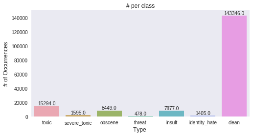
Class Imbalance
- class는 ‘clean’과 ‘clean’이 아닌 toxic 관련 comments가 매우 불균형한 상태 (9:1 정도의 비율)
- class는 multi-tagging 되어 있음
- null data는 존재하지 않음 (train/test 모두)
x=train.iloc[:,2:].sum()
#marking comments without any tags as "clean"
rowsums=train.iloc[:,2:].sum(axis=1)
train['clean']=(rowsums==0)
#count number of clean entries
train['clean'].sum()
print("Total comments = ",len(train))
print("Total clean comments = ",train['clean'].sum())
print("Total tags =",x.sum())
Total comments =  159571
Total clean comments =  143346
Total tags = 35098
print(x)
toxic            15294
severe_toxic      1595
obscene           8449
threat             478
insult            7877
identity_hate     1405
dtype: int64
아래 결과에는 train/test 모두 null data가 없다고 나오지만, 실제로 test data에 “ “로 표현되어 있어서 NA로 잡히지 않는 data가 1개 존재했음
print("Check for missing values in Train dataset")
null_check=train.isnull().sum()
print(null_check)
print("Check for missing values in Test dataset")
null_check=test.isnull().sum()
print(null_check)
print("filling NA with \"unknown\"")
train["comment_text"].fillna("unknown", inplace=True)
test["comment_text"].fillna("unknown", inplace=True)
Check for missing values in Train dataset
id               0
comment_text     0
toxic            0
severe_toxic     0
obscene          0
threat           0
insult           0
identity_hate    0
clean            0
dtype: int64
Check for missing values in Test dataset
id              0
comment_text    0
dtype: int64
filling NA with "unknown"
x=train.iloc[:,2:].sum()
#plot
plt.figure(figsize=(8,4))
ax= sns.barplot(x.index, x.values, alpha=0.8)
plt.title("# per class")
plt.ylabel('# of Occurrences', fontsize=12)
plt.xlabel('Type ', fontsize=12)
#adding the text labels
rects = ax.patches
labels = x.values
for rect, label in zip(rects, labels):
    height = rect.get_height()
    ax.text(rect.get_x() + rect.get_width()/2, height + 5, label, ha='center', va='bottom')

plt.show()
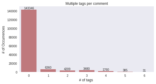
x=rowsums.value_counts()

#plot
plt.figure(figsize=(8,4))
ax = sns.barplot(x.index, x.values, alpha=0.8,color=color[2])
plt.title("Multiple tags per comment")
plt.ylabel('# of Occurrences', fontsize=12)
plt.xlabel('# of tags ', fontsize=12)

#adding the text labels
rects = ax.patches
labels = x.values
for rect, label in zip(rects, labels):
    height = rect.get_height()
    ax.text(rect.get_x() + rect.get_width()/2, height + 5, label, ha='center', va='bottom')

plt.show()
Correlation Plot
Correlation Coefficient
- 상관관계의 정도를 파악하는 상관계수(Correlation coefficient)는 두 변수간의 연관된 정도를 나타낼 뿐 인과관계를 설명하는 것은 아님
- 두 변수간에 원인과 결과의 인과관계가 있는지에 대한 것은 회귀분석을 통해 인과관계의 방향, 정도와 수학적 모델을 확인해야 함
피어슨 상관 계수(Pearson correlation coefficient 또는 Pearson’s r)
- 피어슨 상관 계수 r은 두 변수간의 관련성을 구하기 위해 보편적으로 이용됨
- 연속형 변수 간의 상관관계를 파악할 때 사용(정규분포를 가정하기 때문에 categorical 변수에는 적합하지 않음)
- r = X와 Y가 함께 변하는 정도 / X와 Y가 각각 변하는 정도
스피어만 상관 계수
- 스피어만 상관계수(Spearman correlation coefficient) 는 데이터가 서열척도인 경우 즉 자료의 값 대신 순위를 이용하는 경우의 상관계수(연속형 또는 순서형 변수에 사용 가능)
- 데이터를 작은 것부터 차례로 순위를 매겨 서열 순서로 바꾼 뒤 순위를 이용해 상관계수를 구함
- 두 변수 간의 연관 관계가 있는지 없는지를 밝혀주며 자료에 이상점이 있거나 표본크기가 작을 때 유용
예를 들어, 국어 점수와 영어 점수 간의 상관 계수는 피어슨 상관 계수로, 국어 성적 석차와 영어 성적 석차의 상관 계수는 스피어만 상관 계수로 계산할 수 있다.
temp_df=train.iloc[:,2:-1]
# filter temp by removing clean comments
# temp_df=temp_df[~train.clean]

corr=temp_df.corr()
plt.figure(figsize=(10,8))
sns.heatmap(corr,
            xticklabels=corr.columns.values,
            yticklabels=corr.columns.values, annot=True)
<matplotlib.axes._subplots.AxesSubplot at 0x7f1cd0ddae80>
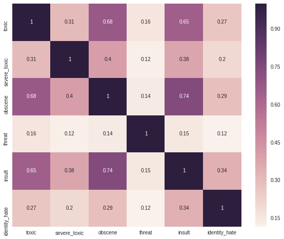
위 그래프는 pandas의 corr 함수를 사용한 correlation plot을 보여주는데, 해당 함수는 pearson 상관 계수 값을 표현함으로 categorical data 상관 계수 파악을 위해 적절하지 않음.
따라서 Cramer’s V statistics로 다시 상관 관계 파악
categorical data의 패턴 분석을 위해 아래와 같은 방법이 쓰일 수 있음
- ConfusionMatrix / Crosstab (co-occuring frequency table)
- Cramer’s V statistics
아래 Crosstab 분석 결과를 보았을 때,
- severe_toxic은 toxic에 모두 포함되고
- clean이 아닌 다른 class는 일부분 데이터를 제외하고 대부분 toxic class와 연관성이 깊다
#Crosstab
# Since technically a crosstab between all 6 classes is impossible to vizualize, lets take a
# look at toxic with other tags
main_col="toxic"
corr_mats=[]
for other_col in temp_df.columns[1:]:
    confusion_matrix = pd.crosstab(temp_df[main_col], temp_df[other_col])
    corr_mats.append(confusion_matrix)
out = pd.concat(corr_mats,axis=1,keys=temp_df.columns[1:])

#cell highlighting
out = out.style.apply(highlight_min,axis=0)
out
#Checking for Toxic and Severe toxic for now

col1="toxic"
col2="severe_toxic"
confusion_matrix = pd.crosstab(temp_df[col1], temp_df[col2])
print("Confusion matrix between toxic and severe toxic:")
print(confusion_matrix)
new_corr=cramers_corrected_stat(confusion_matrix)
print("The correlation between Toxic and Severe toxic using Cramer's stat=",new_corr)
Confusion matrix between toxic and severe toxic:
severe_toxic       0     1
toxic
0             144277     0
1              13699  1595
The correlation between Toxic and Severe toxic using Cramer's stat= 0.308502905405
Toxic comments에 IP, ID, 숫자 나열 등이 포함되어 있음
print("toxic:")
print(train[train.severe_toxic==1].iloc[3,1])
print('\n\n')
print("severe_toxic:")
print(train[train.severe_toxic==1].iloc[4,1])
print('\n\n')
print("Obscene:")
print(train[train.obscene==1].iloc[1,1])
print(train[train.obscene==1].iloc[2,1])
print('\n\n')
print("identity_hate:")
print(train[train.identity_hate==1].iloc[4,1])
#print(train[train.identity_hate==1].iloc[4,1])
toxic:
Hi

Im a fucking bitch.

50.180.208.181


severe_toxic:
What a motherfucking piece of crap those fuckheads for blocking us!


Obscene:
You are gay or antisemmitian?

Archangel WHite Tiger

Meow! Greetingshhh!

Uh, there are two ways, why you do erased my comment about WW2, that holocaust was brutally slaying of Jews and not gays/Gypsys/Slavs/anyone...

1 - If you are anti-semitian, than shave your head bald and go to the skinhead meetings!

2 - If you doubt words of the Bible, that homosexuality is a deadly sin, make a pentagram tatoo on your forehead go to the satanistic masses with your gay pals!

3 - First and last warning, you fucking gay - I won't appreciate if any more nazi shwain would write in my page! I don't wish to talk to you anymore!

Beware of the Dark Side!
FUCK YOUR FILTHY MOTHER IN THE ASS, DRY!


identity_hate:
u r a tw@ fuck off u gay boy.U r smelly.Fuck ur mum poopie
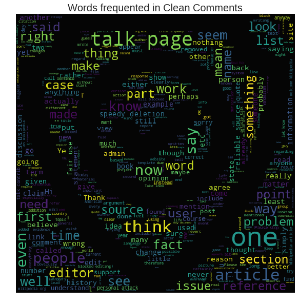
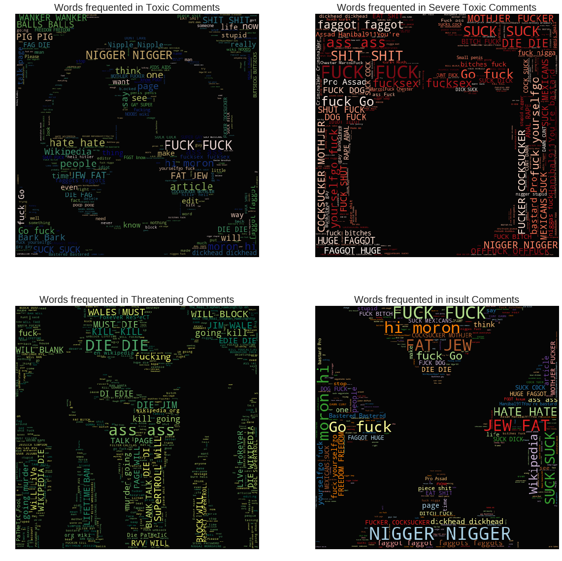
Word Cloud
!ls ./input/imagesforkernal/
stopword=set(STOPWORDS)
#print(stopword)
anger.png	      bomb.png	    megaphone.png  swords.png
biohazard-symbol.png  gas-mask.png  safe-zone.png  toxic-sign.png
print(stopword)
{"they're", 'would', 'a', "can't", "hadn't", 'very', "you'd", 'did', "didn't", 'those', "haven't", 'yourselves', 'her', "i've", 'can', 'over', 'there', "here's", 'no', 'if', 'shall', 'cannot', 'hers', "shan't", "i'll", 'ours', 'since', 'once', 'their', 'been', 'any', 'whom', 'other', "who's", "weren't", 'com', 'as', 'or', 'into', "where's", 'for', 'having', 'else', 'until', 'where', 'be', 'like', 'who', 'why', 'www', 'could', "you've", 'is', 'it', 'theirs', "we'd", 'from', 'of', 'she', 'in', 'through', 'against', 'at', 'myself', 'was', 'they', 'nor', "we'll", 'do', 'the', 'on', 'we', 'am', 'doing', 'were', 'being', 'my', 'most', "we've", "won't", 'otherwise', 'ought', 'you', "he's", 'has', "i'm", "how's", 'yours', "when's", "aren't", 'he', 'how', "don't", "why's", 'had', "doesn't", "she'll", "hasn't", "it's", 'them', "she'd", 'only', 'about', 'i', "what's", 'all', 'before', 'themselves', 'then', 'however', "mustn't", "he'd", 'here', 'me', 'own', 'your', 'below', 'between', 'should', 'does', 'this', "he'll", 'up', "wasn't", 'which', "couldn't", 'down', 'further', "she's", "isn't", 'these', 'not', 'few', 'above', 'herself', 'during', 'get', 'have', "there's", 'because', 'are', 'such', 'with', 'again', "we're", "wouldn't", 'him', 'more', "they'll", 'itself', "they'd", "you'll", "you're", 'http', 'k', 'just', 'its', 'our', 'and', "shouldn't", 'what', 'both', 'r', 'when', 'under', 'so', 'an', 'yourself', 'too', 'out', 'same', 'also', 'ourselves', 'after', 'while', "i'd", 'his', 'that', 'but', 'off', "they've", 'himself', 'by', 'each', "that's", 'some', 'than', 'to', 'ever', "let's"}
#clean comments
clean_mask=np.array(Image.open("./input/imagesforkernal/safe-zone.png"))
clean_mask=clean_mask[:,:,1]
#wordcloud for clean comments
subset=train[train.clean==True]
text=subset.comment_text.values
wc= WordCloud(background_color="black",max_words=2000,mask=clean_mask,stopwords=stopword)
wc.generate(" ".join(text))
plt.figure(figsize=(20,10))
plt.axis("off")
plt.title("Words frequented in Clean Comments", fontsize=20)
plt.imshow(wc.recolor(colormap= 'viridis' , random_state=17), alpha=0.98)
plt.show()
toxic_mask=np.array(Image.open("./input/imagesforkernal/toxic-sign.png"))
toxic_mask=toxic_mask[:,:,1]
#wordcloud for clean comments
subset=train[train.toxic==1]
text=subset.comment_text.values
wc= WordCloud(background_color="black",max_words=4000,mask=toxic_mask,stopwords=stopword)
wc.generate(" ".join(text))
plt.figure(figsize=(20,20))
plt.subplot(221)
plt.axis("off")
plt.title("Words frequented in Toxic Comments", fontsize=20)
plt.imshow(wc.recolor(colormap= 'gist_earth' , random_state=244), alpha=0.98)

#Severely toxic comments
plt.subplot(222)
severe_toxic_mask=np.array(Image.open("./input/imagesforkernal/bomb.png"))
severe_toxic_mask=severe_toxic_mask[:,:,1]
subset=train[train.severe_toxic==1]
text=subset.comment_text.values
wc= WordCloud(background_color="black",max_words=2000,mask=severe_toxic_mask,stopwords=stopword)
wc.generate(" ".join(text))
plt.axis("off")
plt.title("Words frequented in Severe Toxic Comments", fontsize=20)
plt.imshow(wc.recolor(colormap= 'Reds' , random_state=244), alpha=0.98)

#Threat comments
plt.subplot(223)
threat_mask=np.array(Image.open("./input/imagesforkernal/anger.png"))
threat_mask=threat_mask[:,:,1]
subset=train[train.threat==1]
text=subset.comment_text.values
wc= WordCloud(background_color="black",max_words=2000,mask=threat_mask,stopwords=stopword)
wc.generate(" ".join(text))
plt.axis("off")
plt.title("Words frequented in Threatening Comments", fontsize=20)
plt.imshow(wc.recolor(colormap= 'summer' , random_state=2534), alpha=0.98)

#insult
plt.subplot(224)
insult_mask=np.array(Image.open("./input/imagesforkernal/swords.png"))
insult_mask=insult_mask[:,:,1]
subset=train[train.insult==1]
text=subset.comment_text.values
wc= WordCloud(background_color="black",max_words=2000,mask=insult_mask,stopwords=stopword)
wc.generate(" ".join(text))
plt.axis("off")
plt.title("Words frequented in insult Comments", fontsize=20)
plt.imshow(wc.recolor(colormap= 'Paired_r' , random_state=244), alpha=0.98)

plt.show()
Feature Engineering
data를 설명할 수 있을 만한 feature를 더 생성
- count_sent / count_word / count_unique_word / count_letters / count_punctuations
- count_words_upper / count_words_title / count_stopwords / mean_word_len
- word_unique_percent / punc_percent
merge=pd.concat([train.iloc[:,0:2],test.iloc[:,0:2]])
df=merge.reset_index(drop=True)

## Indirect features

#Sentense count in each comment:
    #  '\n' can be used to count the number of sentences in each comment
df['count_sent']=df["comment_text"].apply(lambda x: len(re.findall("\n",str(x)))+1)
#Word count in each comment:
df['count_word']=df["comment_text"].apply(lambda x: len(str(x).split()))
#Unique word count
df['count_unique_word']=df["comment_text"].apply(lambda x: len(set(str(x).split())))
#Letter count
df['count_letters']=df["comment_text"].apply(lambda x: len(str(x)))
#punctuation count
df["count_punctuations"] =df["comment_text"].apply(lambda x: len([c for c in str(x) if c in string.punctuation]))
#upper case words count
df["count_words_upper"] = df["comment_text"].apply(lambda x: len([w for w in str(x).split() if w.isupper()]))
#title case words count
df["count_words_title"] = df["comment_text"].apply(lambda x: len([w for w in str(x).split() if w.istitle()]))
#Number of stopwords
df["count_stopwords"] = df["comment_text"].apply(lambda x: len([w for w in str(x).lower().split() if w in eng_stopwords]))
#Average length of the words
df["mean_word_len"] = df["comment_text"].apply(lambda x: np.mean([len(w) for w in str(x).split()]))
#derived features
#Word count percent in each comment:
df['word_unique_percent']=df['count_unique_word']*100/df['count_word']
#derived features
#Punct percent in each comment:
df['punct_percent']=df['count_punctuations']*100/df['count_word']
#serperate train and test features
train_feats=df.iloc[0:len(train),]
test_feats=df.iloc[len(train):,]
#join the tags
train_tags=train.iloc[:,2:]
train_feats=pd.concat([train_feats,train_tags],axis=1)
train_feats['count_sent'].loc[train_feats['count_sent']>10] = 10
plt.figure(figsize=(12,6))
## sentenses
plt.subplot(121)
plt.suptitle("Are longer comments more toxic?",fontsize=20)
sns.violinplot(y='count_sent',x='clean', data=train_feats,split=True)
plt.xlabel('Clean?', fontsize=12)
plt.ylabel('# of sentences', fontsize=12)
plt.title("Number of sentences in each comment", fontsize=15)
# words
train_feats['count_word'].loc[train_feats['count_word']>200] = 200
plt.subplot(122)
sns.violinplot(y='count_word',x='clean', data=train_feats,split=True,inner="quart")
plt.xlabel('Clean?', fontsize=12)
plt.ylabel('# of words', fontsize=12)
plt.title("Number of words in each comment", fontsize=15)

plt.show()
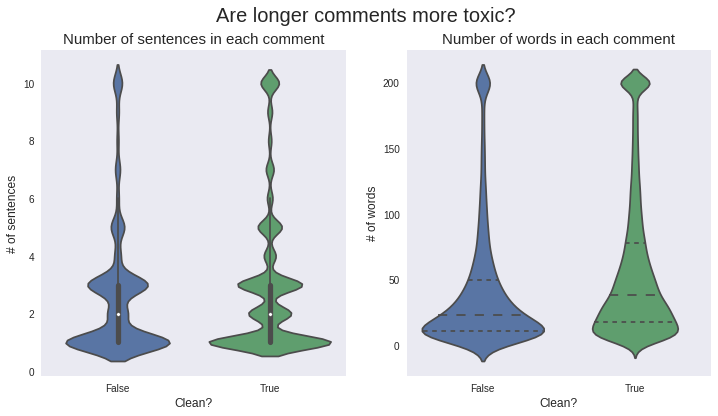
문장 길이, 한 문장 안에 포함되는 단어 개수는 toxic 여부와 크게 상관성이 없다.
violin plot은 기존의 box plot을 대체, 중간값, 4분위 표시 등이 가능하고 각 위치의 비율 (해당 count / 전체 count) 포함
train_feats['count_unique_word'].loc[train_feats['count_unique_word']>200] = 200
#prep for split violin plots
#For the desired plots , the data must be in long format
temp_df = pd.melt(train_feats, value_vars=['count_word', 'count_unique_word'], id_vars='clean')
#spammers - comments with less than 40% unique words
spammers=train_feats[train_feats['word_unique_percent']<30]
plt.figure(figsize=(16,12))
plt.suptitle("What's so unique ?",fontsize=20)
gridspec.GridSpec(2,2)
plt.subplot2grid((2,2),(0,0))
sns.violinplot(x='variable', y='value', hue='clean', data=temp_df,split=True,inner='quartile')
plt.title("Absolute wordcount and unique words count")
plt.xlabel('Feature', fontsize=12)
plt.ylabel('Count', fontsize=12)

plt.subplot2grid((2,2),(0,1))
plt.title("Percentage of unique words of total words in comment")
#sns.boxplot(x='clean', y='word_unique_percent', data=train_feats)
ax=sns.kdeplot(train_feats[train_feats.clean == 0].word_unique_percent, label="Bad",shade=True,color='r')
ax=sns.kdeplot(train_feats[train_feats.clean == 1].word_unique_percent, label="Clean")
plt.legend()
plt.ylabel('Number of occurances', fontsize=12)
plt.xlabel('Percent unique words', fontsize=12)

x=spammers.iloc[:,-7:].sum()
plt.subplot2grid((2,2),(1,0),colspan=2)
plt.title("Count of comments with low(<30%) unique words",fontsize=15)
ax=sns.barplot(x=x.index, y=x.values,color=color[3])

#adding the text labels
rects = ax.patches
labels = x.values
for rect, label in zip(rects, labels):
    height = rect.get_height()
    ax.text(rect.get_x() + rect.get_width()/2, height + 5, label, ha='center', va='bottom')

plt.xlabel('Threat class', fontsize=12)
plt.ylabel('# of comments', fontsize=12)
plt.show()
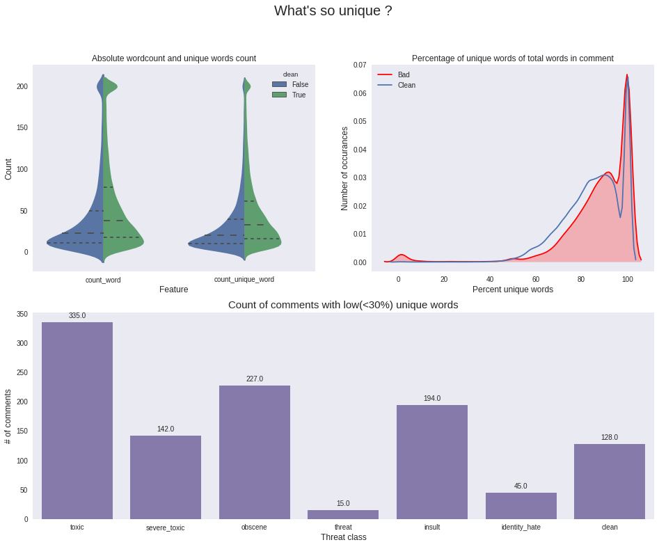
Word count VS unique word count Features
- word count와 unique word count feature에 대해서는 clean/toxic comment 간 차이가 있는 것을 확인할 수 있음
- count / unique count word가 30 이하인 comment에 대해 toxic 관련 밀도가 높은 것을 확인할 수 있음
- unique word가 30개 이하인 comment만 뽑아서 보았을 때 toxic 관련 비율이 월등이 높음 (전체 데이터 셋에서 clean data set이 90% 이상임에도 불구하고)
spammer feature 또한 toxic 성격을 더 가지고 있지만 spammer comments 안에 normal word도 포함되기 때문에 이것을 모델에 반영하기에는 위험성이 있음 (예를 들어 mitt romney라는 단어를 toxic word로 규정할 가능성이 있기 때문에)
print("Clean Spam example:")
print(spammers[spammers.clean==1].comment_text.iloc[1])
print("Toxic Spam example:")
print(spammers[spammers.toxic==1].comment_text.iloc[2])
Clean Spam example:
Towns and Villages in Ark-La-Tex]]
 Cities, boroughs and towns in the Republic of Ireland
 Cities, boroughs, and townships along the Susquehanna River
 Cities, towns and villages in Alborz Province
 Cities, towns and villages in Ardabil Province
 Cities, towns and villages in Bhutan
 Cities, towns and villages in Bushehr Province
 Cities, towns and villages in Chaharmahal and Bakhtiari Province
 Cities, towns and villages in Cyprus
 Cities, towns and villages in Dutch Limburg
 Cities, towns and villages in East Azerbaijan Province
 Cities, towns and villages in East Timor
 Cities, towns and villages in Fars Province
 Cities, towns and villages in Flevoland
 Cities, towns and villages in Friesland
 Cities, towns and villages in Gelderland
 Cities, towns and villages in Gilan Province
 Cities, towns and villages in Golestan Province
 Cities, towns and villages in Groningen
 Cities, towns and villages in Hamadan Province
 Cities, towns and villages in Hormozgan Province
 Cities, towns and villages in Ilam Province
 Cities, towns and villages in Isfahan Province
 Cities, towns and villages in Kerman Province
 Cities, towns and villages in Kermanshah Province
 Cities, towns and villages in Khuzestan Province
 Cities, towns and villages in Kohgiluyeh and Boyer-Ahmad Province
 Cities, towns and villages in Kurdistan Province
 Cities, towns and villages in Lorestan Province
 Cities, towns and villages in Markazi Province
 Cities, towns and villages in Mazandaran Province
 Cities, towns and villages in North Brabant
 Cities, towns and villages in North Holland
 Cities, towns and villages in North Khorasan Province
 Cities, towns and villages in Overijssel
 Cities, towns and villages in Qazvin Province
 Cities, towns and villages in Qom Province
 Cities, towns and villages in Razavi Khorasan Province
 Cities, towns and villages in Saint Vincent and the Grenadines
 Cities, towns and villages in Samoa
 Cities, towns and villages in Semnan Province
 Cities, towns and villages in Sistan and Baluchestan Province
 Cities, towns and villages in South Holland
 Cities, towns and villages in South Khorasan Province
 Cities, towns and villages in Tehran Province
 Cities, towns and villages in Turkmenistan
 Cities, towns and villages in Utrecht
 Cities, towns and villages in Vojvodina
 Cities, towns and villages in West Azerbaijan Province
 Cities, towns and villages in Yazd Province
 Cities, towns and villages in Zanjan Province
 Cities, towns and villages in Zeeland
 Cities, towns and villages in the Maldives
 Cities, towns and villages in the Solomon Islands
 Cities, towns, and villages in Békés county
 Cities, towns, and villages in Louisiana
Toxic Spam example:
User:NHRHS2010 is a homo like mitt romney is.
User:NHRHS2010 is a homo like mitt romney is.
 User:Enigmaman is a homo like mitt romney is.
User:Enigmaman is a homo like mitt romney is.
 User:NHRHS2010 is a homo like mitt romney is.
User:NHRHS2010 is a homo like mitt romney is.
 User:Enigmaman is a homo like mitt romney is.
User:Enigmaman is a homo like mitt romney is.== User:NHRHS2010 is a homo like mitt romney is. ==
User:NHRHS2010 is a homo like mitt romney is.
 User:Enigmaman is a homo like mitt romney is.
User:Enigmaman is a homo like mitt romney is.== User:NHRHS2010 is a homo like mitt romney is. ==
User:NHRHS2010 is a homo like mitt romney is.
 User:Enigmaman is a homo like mitt romney is.
User:Enigmaman is a homo like mitt romney is.== User:NHRHS2010 is a homo like mitt romney is. ==
User:NHRHS2010 is a homo like mitt romney is.
 User:Enigmaman is a homo like mitt romney is.
User:Enigmaman is a homo like mitt romney is.== User:NHRHS2010 is a homo like mitt romney is. ==
User:NHRHS2010 is a homo like mitt romney is.
 User:Enigmaman is a homo like mitt romney is.
User:Enigmaman is a homo like mitt romney is.== User:NHRHS2010 is a homo like mitt romney is. ==
User:NHRHS2010 is a homo like mitt romney is.
 User:Enigmaman is a homo like mitt romney is.
User:Enigmaman is a homo like mitt romney is.== User:NHRHS2010 is a homo like mitt romney is. ==
User:NHRHS2010 is a homo like mitt romney is.
 User:Enigmaman is a homo like mitt romney is.
User:Enigmaman is a homo like mitt romney is.== User:NHRHS2010 is a homo like mitt romney is. ==
User:NHRHS2010 is a homo like mitt romney is.
 User:Enigmaman is a homo like mitt romney is.
User:Enigmaman is a homo like mitt romney is.== User:NHRHS2010 is a homo like mitt romney is. ==
User:NHRHS2010 is a homo like mitt romney is.
 User:Enigmaman is a homo like mitt romney is.
User:Enigmaman is a homo like mitt romney is.== User:NHRHS2010 is a homo like mitt romney is. ==
User:NHRHS2010 is a homo like mitt romney is.
 User:Enigmaman is a homo like mitt romney is.
User:Enigmaman is a homo like mitt romney is.== User:NHRHS2010 is a homo like mitt romney is. ==
User:NHRHS2010 is a homo like mitt romney is.
 User:Enigmaman is a homo like mitt romney is.
User:Enigmaman is a homo like mitt romney is.== User:NHRHS2010 is a homo like mitt romney is. ==
User:NHRHS2010 is a homo like mitt romney is.
 User:Enigmaman is a homo like mitt romney is.
User:Enigmaman is a homo like mitt romney is.== User:NHRHS2010 is a homo like mitt romney is. ==
User:NHRHS2010 is a homo like mitt romney is.
 User:Enigmaman is a homo like mitt romney is.
User:Enigmaman is a homo like mitt romney is.== User:NHRHS2010 is a homo like mitt romney is. ==
User:NHRHS2010 is a homo like mitt romney is.
 User:Enigmaman is a homo like mitt romney is.
User:Enigmaman is a homo like mitt romney is.== User:NHRHS2010 is a homo like mitt romney is. ==
User:NHRHS2010 is a homo like mitt romney is.
 User:Enigmaman is a homo like mitt romney is.
User:Enigmaman is a homo like mitt romney is.== User:NHRHS2010 is a homo like mitt romney is. ==
User:NHRHS2010 is a homo like mitt romney is.
 User:Enigmaman is a homo like mitt romney is.
User:Enigmaman is a homo like mitt romney is.== User:NHRHS2010 is a homo like mitt romney is. ==
User:NHRHS2010 is a homo like mitt romney is.
 User:Enigmaman is a homo like mitt romney is.
User:Enigmaman is a homo like mitt romney is.== User:NHRHS2010 is a homo like mitt romney is. ==
User:NHRHS2010 is a homo like mitt romney is.
 User:Enigmaman is a homo like mitt romney is.
User:Enigmaman is a homo like mitt romney is.== User:NHRHS2010 is a homo like mitt romney is. ==
User:NHRHS2010 is a homo like mitt romney is.
 User:Enigmaman is a homo like mitt romney is.
User:Enigmaman is a homo like mitt romney is.== User:NHRHS2010 is a homo like mitt romney is. ==
User:NHRHS2010 is a homo like mitt romney is.
 User:Enigmaman is a homo like mitt romney is.
User:Enigmaman is a homo like mitt romney is.== User:NHRHS2010 is a homo like mitt romney is. ==
User:NHRHS2010 is a homo like mitt romney is.
 User:Enigmaman is a homo like mitt romney is. NEWL
Leaky feature
- ip / count_ip / link / count_links / article_id / article_id_flag / username / count_username
feature engineering 할 때 direct feature 보다 indirect / leaky feature를 먼저 생성하고 확인해보는 것이 좋음
direct feature (count 관련 features)는 clean corpus에서 유효하고, leaky feature은 데이터 전처리에서 발생할 수 있는 정보 손실에 대해 보충해 줄 수 있는 역할을 할 수 있음
#Leaky features
df['ip']=df["comment_text"].apply(lambda x: re.findall("\d{1,3}\.\d{1,3}\.\d{1,3}\.\d{1,3}",str(x)))
#count of ip addresses
df['count_ip']=df["ip"].apply(lambda x: len(x))

#links
df['link']=df["comment_text"].apply(lambda x: re.findall("http://.*com",str(x)))
#count of links
df['count_links']=df["link"].apply(lambda x: len(x))

#article ids
df['article_id']=df["comment_text"].apply(lambda x: re.findall("\d:\d\d\s{0,5}$",str(x)))
df['article_id_flag']=df.article_id.apply(lambda x: len(x))

#username
##              regex for     Match anything with [[User: ---------- ]]
# regexp = re.compile("\[\[User:(.*)\|")
df['username']=df["comment_text"].apply(lambda x: re.findall("\[\[User(.*)\|",str(x)))
#count of username mentions
df['count_usernames']=df["username"].apply(lambda x: len(x))
#check if features are created
#df.username[df.count_usernames>0]

# Leaky Ip
cv = CountVectorizer()
count_feats_ip = cv.fit_transform(df["ip"].apply(lambda x : str(x)))


# Leaky usernames

cv = CountVectorizer()
count_feats_user = cv.fit_transform(df["username"].apply(lambda x : str(x)))
df[df.count_usernames!=0].comment_text.iloc[0]
'2010]]\n[[User talk:Wikireader41/Archive4|Archive 5-Mar 15'
# check few names
cv.get_feature_names()[120:130]
['destruction',
 'diablo',
 'diligent',
 'dland',
 'dlohcierekim',
 'dodo',
 'dominick',
 'douglas',
 'dpl',
 'dr']
leaky_feats=df[["ip","link","article_id","username","count_ip","count_links","count_usernames","article_id_flag"]]
leaky_feats_train=leaky_feats.iloc[:train.shape[0]]
leaky_feats_test=leaky_feats.iloc[train.shape[0]:]
#filterout the entries without ips
train_ips=leaky_feats_train.ip[leaky_feats_train.count_ip!=0]
test_ips=leaky_feats_test.ip[leaky_feats_test.count_ip!=0]
#get the unique list of ips in test and train datasets
train_ip_list=list(set([a for b in train_ips.tolist() for a in b]))
test_ip_list=list(set([a for b in test_ips.tolist() for a in b]))
# get common elements
common_ip_list=list(set(train_ip_list).intersection(test_ip_list))
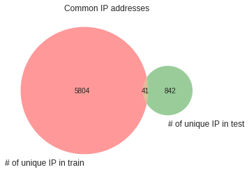
plt.title("Common IP addresses")
venn.venn2(subsets=(len(train_ip_list),len(test_ip_list),len(common_ip_list)),set_labels=("# of unique IP in train","# of unique IP in test"))
plt.show()
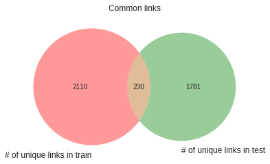
#filterout the entries without links
train_links=leaky_feats_train.link[leaky_feats_train.count_links!=0]
test_links=leaky_feats_test.link[leaky_feats_test.count_links!=0]
#get the unique list of ips in test and train datasets
train_links_list=list(set([a for b in train_links.tolist() for a in b]))
test_links_list=list(set([a for b in test_links.tolist() for a in b]))

# get common elements
common_links_list=list(set(train_links_list).intersection(test_links_list))
plt.title("Common links")
venn.venn2(subsets=(len(train_links_list),len(test_links_list),len(common_links_list)),
           set_labels=("# of unique links in train","# of unique links in test"))
plt.show()
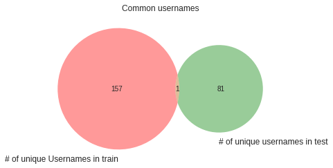
#filterout the entries without users
train_users=leaky_feats_train.username[leaky_feats_train.count_usernames!=0]
test_users=leaky_feats_test.username[leaky_feats_test.count_usernames!=0]
#get the unique list of ips in test and train datasets
train_users_list=list(set([a for b in train_users.tolist() for a in b]))
test_users_list=list(set([a for b in test_users.tolist() for a in b]))

# get common elements
common_users_list=list(set(train_users_list).intersection(test_users_list))
plt.title("Common usernames")
venn.venn2(subsets=(len(train_users_list),len(test_users_list),len(common_users_list)),
           set_labels=("# of unique Usernames in train","# of unique usernames in test"))
plt.show()
train_ip_list=list(set([a for b in train_ips.tolist() for a in b]))
test_ip_list=list(set([a for b in test_ips.tolist() for a in b]))

# get common elements
blocked_ip_list_train=list(set(train_ip_list).intersection(blocked_ips))
blocked_ip_list_test=list(set(test_ip_list).intersection(blocked_ips))

print("There are",len(blocked_ip_list_train),"blocked IPs in train dataset")
print("There are",len(blocked_ip_list_test),"blocked IPs in test dataset")
There are 6 blocked IPs in train dataset
There are 0 blocked IPs in test dataset
end_time=time.time()
print("total time till Leaky feats",end_time-start_time)
total time till Leaky feats 5089.553529024124
unique ip / link가 train / test 데이터에서 중복되는 것이 있으므로 feature engineering에서 사용 가능 (username은 겹치는 것이 한 개 밖에 없음)
wikipedia에서 받아온 blocked ip도 train dataset에서 6개 발견됨
Corpus Cleansing
corpus=merge.comment_text
print(corpus.iloc[12235])
print('\n\n')
print(clean(corpus.iloc[12235]))
"

 NOTE If you read above, and follow the links, any reader can see that I cited correctly the links I added on this subject. Vidkun has added anotations to make them read as the oposite, but these links show the ""official"" line taken by UGLE. I will not be trapped by any User into so-called 3RR, so he can peddle his POV. Strangly, ALL other ""MASONS"" are quiet, leaving ‘‘me’’ to defend that factual truth on my own. ""Thanks"" Brethren. Sitting any blocking out if given...  "


" note read , follow link , reader see cite correctly link add subject . vidkun add anotations make read oposite , link show " " official " " line take ugle . trap user so-called 3rr , peddle pov . strangly , " " masons " " quiet , leave ‘ ‘ ’ ’ defend factual truth . " " thank " " brethren . sit block give ... "
clean_corpus=corpus.apply(lambda x :clean(x))

end_time=time.time()
print("total time till Cleaning",end_time-start_time)
total time till Cleaning 9700.285007715225
# To do next:
# Slang lookup dictionary for sentiments
#http://slangsd.com/data/SlangSD.zip
#http://arxiv.org/abs/1608.05129
# dict lookup
#https://bytes.com/topic/python/answers/694819-regular-expression-dictionary-key-search
Direct features (uni-gram)
count 관련 direct feature를 생성하기 위해 아래와 같은 방법 사용 가능
- CountVectorizer
- TF-IDF Vectorizer
- HashingVectorizer : vocabulary에 대해서 dictionary 대신 hashmap 제공, scalable & faster
### Unigrams -- TF-IDF
# using settings recommended here for TF-IDF -- https://www.kaggle.com/abhishek/approaching-almost-any-nlp-problem-on-kaggle

#some detailed description of the parameters
# min_df=10 --- ignore terms that appear lesser than 10 times
# max_features=None  --- Create as many words as present in the text corpus
    # changing max_features to 10k for memmory issues
# analyzer='word'  --- Create features from words (alternatively char can also be used)
# ngram_range=(1,1)  --- Use only one word at a time (unigrams)
# strip_accents='unicode' -- removes accents
# use_idf=1,smooth_idf=1 --- enable IDF
# sublinear_tf=1   --- Apply sublinear tf scaling, i.e. replace tf with 1 + log(tf)


#temp settings to min=200 to facilitate top features section to run in kernals
#change back to min=10 to get better results
start_unigrams=time.time()
tfv = TfidfVectorizer(min_df=200,  max_features=10000,
            strip_accents='unicode', analyzer='word',ngram_range=(1,1),
            use_idf=1,smooth_idf=1,sublinear_tf=1,
            stop_words = 'english')
tfv.fit(clean_corpus)
features = np.array(tfv.get_feature_names())

train_unigrams =  tfv.transform(clean_corpus.iloc[:train.shape[0]])
test_unigrams = tfv.transform(clean_corpus.iloc[train.shape[0]:])
#get top n for unigrams
tfidf_top_n_per_lass=top_feats_by_class(train_unigrams,features)

end_unigrams=time.time()

print("total time in unigrams",end_unigrams-start_unigrams)
print("total time till unigrams",end_unigrams-start_time)
total time in unigrams 65.25758147239685
total time till unigrams 9778.263393878937
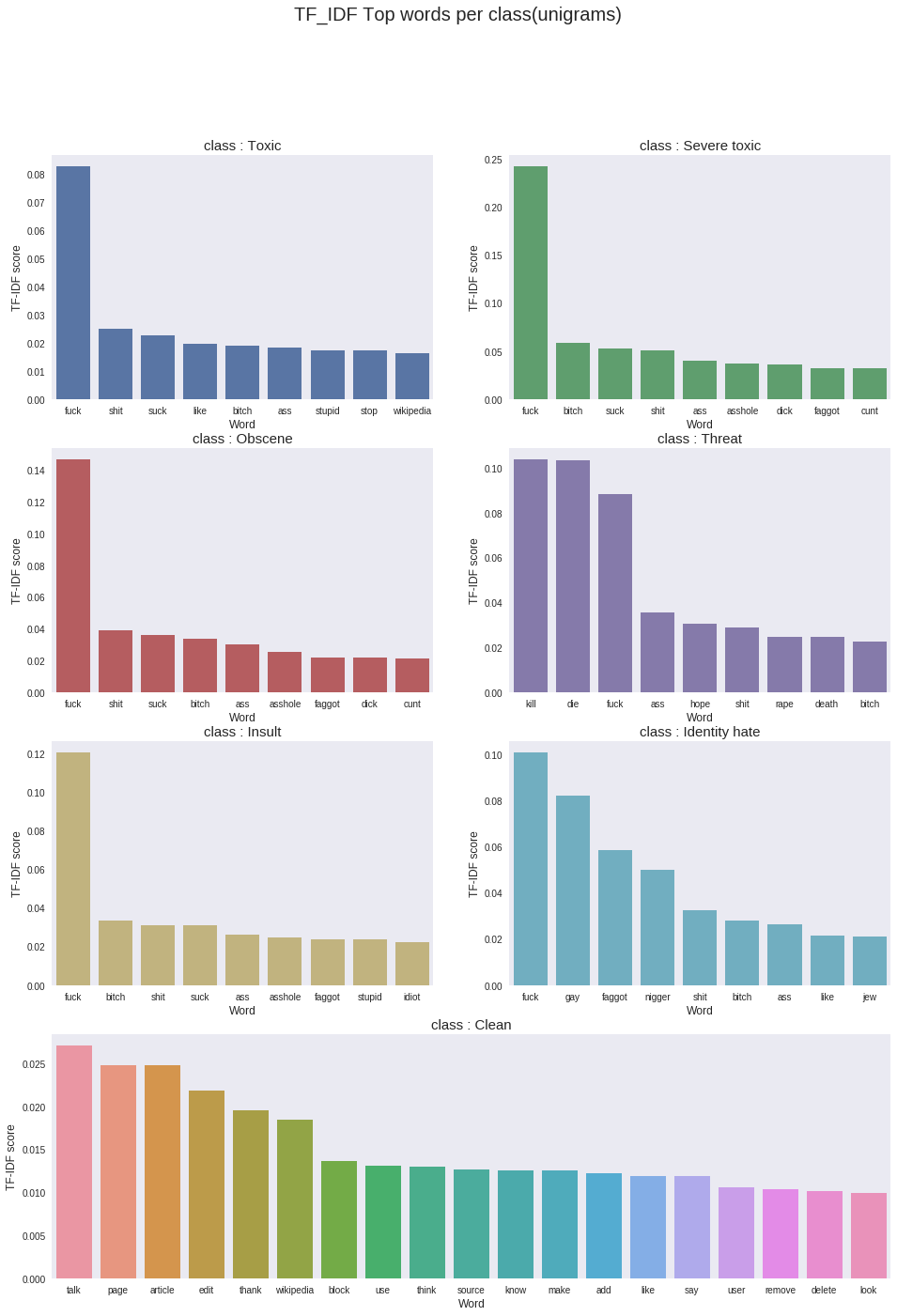
plt.figure(figsize=(16,22))
plt.suptitle("TF_IDF Top words per class(unigrams)",fontsize=20)
gridspec.GridSpec(4,2)
plt.subplot2grid((4,2),(0,0))
sns.barplot(tfidf_top_n_per_lass[0].feature.iloc[0:9],tfidf_top_n_per_lass[0].tfidf.iloc[0:9],color=color[0])
plt.title("class : Toxic",fontsize=15)
plt.xlabel('Word', fontsize=12)
plt.ylabel('TF-IDF score', fontsize=12)

plt.subplot2grid((4,2),(0,1))
sns.barplot(tfidf_top_n_per_lass[1].feature.iloc[0:9],tfidf_top_n_per_lass[1].tfidf.iloc[0:9],color=color[1])
plt.title("class : Severe toxic",fontsize=15)
plt.xlabel('Word', fontsize=12)
plt.ylabel('TF-IDF score', fontsize=12)


plt.subplot2grid((4,2),(1,0))
sns.barplot(tfidf_top_n_per_lass[2].feature.iloc[0:9],tfidf_top_n_per_lass[2].tfidf.iloc[0:9],color=color[2])
plt.title("class : Obscene",fontsize=15)
plt.xlabel('Word', fontsize=12)
plt.ylabel('TF-IDF score', fontsize=12)


plt.subplot2grid((4,2),(1,1))
sns.barplot(tfidf_top_n_per_lass[3].feature.iloc[0:9],tfidf_top_n_per_lass[3].tfidf.iloc[0:9],color=color[3])
plt.title("class : Threat",fontsize=15)
plt.xlabel('Word', fontsize=12)
plt.ylabel('TF-IDF score', fontsize=12)


plt.subplot2grid((4,2),(2,0))
sns.barplot(tfidf_top_n_per_lass[4].feature.iloc[0:9],tfidf_top_n_per_lass[4].tfidf.iloc[0:9],color=color[4])
plt.title("class : Insult",fontsize=15)
plt.xlabel('Word', fontsize=12)
plt.ylabel('TF-IDF score', fontsize=12)


plt.subplot2grid((4,2),(2,1))
sns.barplot(tfidf_top_n_per_lass[5].feature.iloc[0:9],tfidf_top_n_per_lass[5].tfidf.iloc[0:9],color=color[5])
plt.title("class : Identity hate",fontsize=15)
plt.xlabel('Word', fontsize=12)
plt.ylabel('TF-IDF score', fontsize=12)


plt.subplot2grid((4,2),(3,0),colspan=2)
sns.barplot(tfidf_top_n_per_lass[6].feature.iloc[0:19],tfidf_top_n_per_lass[6].tfidf.iloc[0:19])
plt.title("class : Clean",fontsize=15)
plt.xlabel('Word', fontsize=12)
plt.ylabel('TF-IDF score', fontsize=12)

plt.show()
#temp settings to min=150 to facilitate top features section to run in kernals
#change back to min=10 to get better results
tfv = TfidfVectorizer(min_df=150,  max_features=30000,
            strip_accents='unicode', analyzer='word',ngram_range=(2,2),
            use_idf=1,smooth_idf=1,sublinear_tf=1,
            stop_words = 'english')

tfv.fit(clean_corpus)
features = np.array(tfv.get_feature_names())
train_bigrams =  tfv.transform(clean_corpus.iloc[:train.shape[0]])
test_bigrams = tfv.transform(clean_corpus.iloc[train.shape[0]:])
#get top n for bigrams
tfidf_top_n_per_lass=top_feats_by_class(train_bigrams,features)
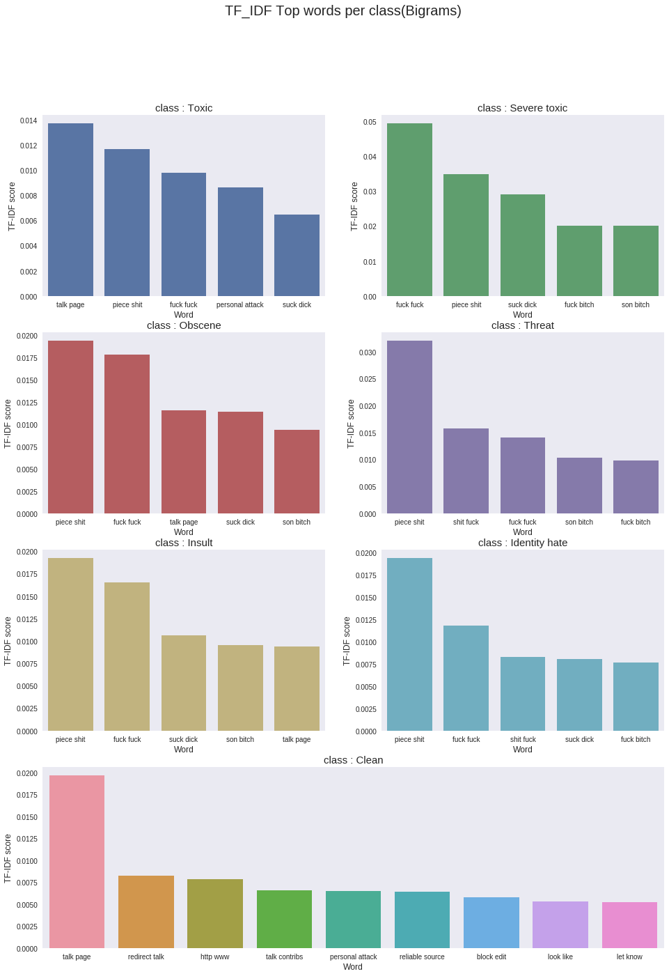
plt.figure(figsize=(16,22))
plt.suptitle("TF_IDF Top words per class(Bigrams)",fontsize=20)
gridspec.GridSpec(4,2)
plt.subplot2grid((4,2),(0,0))
sns.barplot(tfidf_top_n_per_lass[0].feature.iloc[0:5],tfidf_top_n_per_lass[0].tfidf.iloc[0:5],color=color[0])
plt.title("class : Toxic",fontsize=15)
plt.xlabel('Word', fontsize=12)
plt.ylabel('TF-IDF score', fontsize=12)

plt.subplot2grid((4,2),(0,1))
sns.barplot(tfidf_top_n_per_lass[1].feature.iloc[0:5],tfidf_top_n_per_lass[1].tfidf.iloc[0:5],color=color[1])
plt.title("class : Severe toxic",fontsize=15)
plt.xlabel('Word', fontsize=12)
plt.ylabel('TF-IDF score', fontsize=12)


plt.subplot2grid((4,2),(1,0))
sns.barplot(tfidf_top_n_per_lass[2].feature.iloc[0:5],tfidf_top_n_per_lass[2].tfidf.iloc[0:5],color=color[2])
plt.title("class : Obscene",fontsize=15)
plt.xlabel('Word', fontsize=12)
plt.ylabel('TF-IDF score', fontsize=12)


plt.subplot2grid((4,2),(1,1))
sns.barplot(tfidf_top_n_per_lass[3].feature.iloc[0:5],tfidf_top_n_per_lass[3].tfidf.iloc[0:5],color=color[3])
plt.title("class : Threat",fontsize=15)
plt.xlabel('Word', fontsize=12)
plt.ylabel('TF-IDF score', fontsize=12)


plt.subplot2grid((4,2),(2,0))
sns.barplot(tfidf_top_n_per_lass[4].feature.iloc[0:5],tfidf_top_n_per_lass[4].tfidf.iloc[0:5],color=color[4])
plt.title("class : Insult",fontsize=15)
plt.xlabel('Word', fontsize=12)
plt.ylabel('TF-IDF score', fontsize=12)


plt.subplot2grid((4,2),(2,1))
sns.barplot(tfidf_top_n_per_lass[5].feature.iloc[0:5],tfidf_top_n_per_lass[5].tfidf.iloc[0:5],color=color[5])
plt.title("class : Identity hate",fontsize=15)
plt.xlabel('Word', fontsize=12)
plt.ylabel('TF-IDF score', fontsize=12)


plt.subplot2grid((4,2),(3,0),colspan=2)
sns.barplot(tfidf_top_n_per_lass[6].feature.iloc[0:9],tfidf_top_n_per_lass[6].tfidf.iloc[0:9])
plt.title("class : Clean",fontsize=15)
plt.xlabel('Word', fontsize=12)
plt.ylabel('TF-IDF score', fontsize=12)

plt.show()
end_time=time.time()
print("total time till bigrams",end_time-start_time)
total time till bigrams 9908.182485342026
tfv = TfidfVectorizer(min_df=100,  max_features=30000,
            strip_accents='unicode', analyzer='char',ngram_range=(1,4),
            use_idf=1,smooth_idf=1,sublinear_tf=1,
            stop_words = 'english')

tfv.fit(clean_corpus)
features = np.array(tfv.get_feature_names())
train_charngrams =  tfv.transform(clean_corpus.iloc[:train.shape[0]])
test_charngrams = tfv.transform(clean_corpus.iloc[train.shape[0]:])
end_time=time.time()
print("total time till charngrams",end_time-start_time)
total time till charngrams 10267.063734769821
Baseline Model
SELECTED_COLS=['count_sent', 'count_word', 'count_unique_word',
       'count_letters', 'count_punctuations', 'count_words_upper',
       'count_words_title', 'count_stopwords', 'mean_word_len',
       'word_unique_percent', 'punct_percent']
target_x=train_feats[SELECTED_COLS]
# target_x

TARGET_COLS=['toxic', 'severe_toxic', 'obscene', 'threat', 'insult', 'identity_hate']
target_y=train_tags[TARGET_COLS]

# Strat k fold due to imbalanced classes
# split = StratifiedKFold(n_splits=2, random_state=1)

#https://www.kaggle.com/yekenot/toxic-regression
#Just the indirect features -- meta features
print("Using only Indirect features")
model = LogisticRegression(C=3)
X_train, X_valid, y_train, y_valid = train_test_split(target_x, target_y, test_size=0.33, random_state=2018)
train_loss = []
valid_loss = []
importance=[]
preds_train = np.zeros((X_train.shape[0], len(y_train)))
preds_valid = np.zeros((X_valid.shape[0], len(y_valid)))
for i, j in enumerate(TARGET_COLS):
    print('Class:= '+j)
    model.fit(X_train,y_train[j])
    preds_valid[:,i] = model.predict_proba(X_valid)[:,1]
    preds_train[:,i] = model.predict_proba(X_train)[:,1]
    train_loss_class=log_loss(y_train[j],preds_train[:,i])
    valid_loss_class=log_loss(y_valid[j],preds_valid[:,i])
    print('Trainloss=log loss:', train_loss_class)
    print('Validloss=log loss:', valid_loss_class)
    importance.append(model.coef_)
    train_loss.append(train_loss_class)
    valid_loss.append(valid_loss_class)
print('mean column-wise log loss:Train dataset', np.mean(train_loss))
print('mean column-wise log loss:Validation dataset', np.mean(valid_loss))

end_time=time.time()
print("total time till Indirect feat model",end_time-start_time)
Using only Indirect features
Class:= toxic
Trainloss=log loss: 0.301237967533
Validloss=log loss: 0.30032310643
Class:= severe_toxic
Trainloss=log loss: 0.0504951244796
Validloss=log loss: 0.0516744563043
Class:= obscene
Trainloss=log loss: 0.199751128693
Validloss=log loss: 0.198056892129
Class:= threat
Trainloss=log loss: 0.0197706692938
Validloss=log loss: 0.0192285118749
Class:= insult
Trainloss=log loss: 0.188593425839
Validloss=log loss: 0.189818523181
Class:= identity_hate
Trainloss=log loss: 0.0478277367533
Validloss=log loss: 0.0513427824
mean column-wise log loss:Train dataset 0.134612675432
mean column-wise log loss:Validation dataset 0.135074045387
total time till Indirect feat model 10528.657516002655
importance[0][0]
array([  3.68238420e-02,   1.36417093e-05,  -2.23852462e-02,
         2.11721313e-04,   1.33385156e-03,   5.04105088e-02,
        -1.80732670e-02,   4.57792577e-03,  -1.57922696e-03,
        -7.85326544e-03,  -2.75729242e-05])
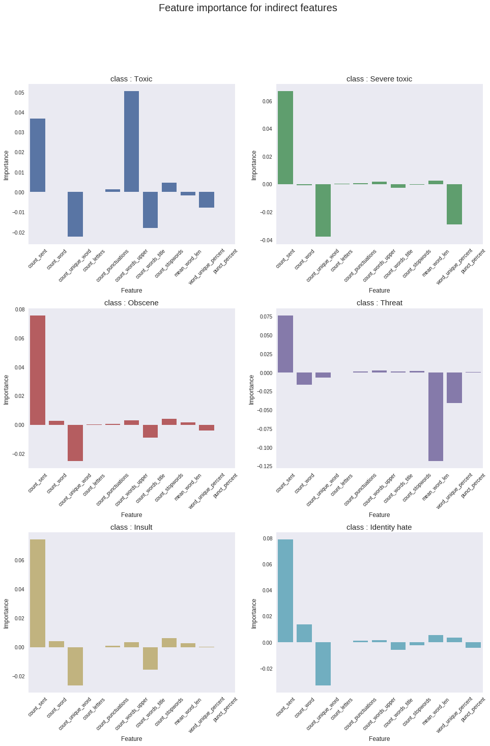
plt.figure(figsize=(16,22))
plt.suptitle("Feature importance for indirect features",fontsize=20)
gridspec.GridSpec(3,2)
plt.subplots_adjust(hspace=0.4)
plt.subplot2grid((3,2),(0,0))
sns.barplot(SELECTED_COLS,importance[0][0],color=color[0])
plt.title("class : Toxic",fontsize=15)
locs, labels = plt.xticks()
plt.setp(labels, rotation=45)
plt.xlabel('Feature', fontsize=12)
plt.ylabel('Importance', fontsize=12)

plt.subplot2grid((3,2),(0,1))
sns.barplot(SELECTED_COLS,importance[1][0],color=color[1])
plt.title("class : Severe toxic",fontsize=15)
locs, labels = plt.xticks()
plt.setp(labels, rotation=45)
plt.xlabel('Feature', fontsize=12)
plt.ylabel('Importance', fontsize=12)

plt.subplot2grid((3,2),(1,0))
sns.barplot(SELECTED_COLS,importance[2][0],color=color[2])
plt.title("class : Obscene",fontsize=15)
locs, labels = plt.xticks()
plt.setp(labels, rotation=45)
plt.xlabel('Feature', fontsize=12)
plt.ylabel('Importance', fontsize=12)


plt.subplot2grid((3,2),(1,1))
sns.barplot(SELECTED_COLS,importance[3][0],color=color[3])
plt.title("class : Threat",fontsize=15)
locs, labels = plt.xticks()
plt.setp(labels, rotation=45)
plt.xlabel('Feature', fontsize=12)
plt.ylabel('Importance', fontsize=12)


plt.subplot2grid((3,2),(2,0))
sns.barplot(SELECTED_COLS,importance[4][0],color=color[4])
plt.title("class : Insult",fontsize=15)
locs, labels = plt.xticks()
plt.setp(labels, rotation=45)
plt.xlabel('Feature', fontsize=12)
plt.ylabel('Importance', fontsize=12)


plt.subplot2grid((3,2),(2,1))
sns.barplot(SELECTED_COLS,importance[5][0],color=color[5])
plt.title("class : Identity hate",fontsize=15)
locs, labels = plt.xticks()
plt.setp(labels, rotation=45)
plt.xlabel('Feature', fontsize=12)
plt.ylabel('Importance', fontsize=12)


# plt.subplot2grid((4,2),(3,0),colspan=2)
# sns.barplot(SELECTED_COLS,importance[6][0],color=color[0])
# plt.title("class : Clean",fontsize=15)
# locs, labels = plt.xticks()
# plt.setp(labels, rotation=90)
# plt.xlabel('Feature', fontsize=12)
# plt.ylabel('Importance', fontsize=12)

plt.show()
from scipy.sparse import csr_matrix, hstack

#Using all direct features
print("Using all features except leaky ones")
target_x = hstack((train_bigrams,train_charngrams,train_unigrams,train_feats[SELECTED_COLS])).tocsr()


end_time=time.time()
print("total time till Sparse mat creation",end_time-start_time)
Using all features except leaky ones
total time till Sparse mat creation 6182.611257553101
model = NbSvmClassifier(C=4, dual=True, n_jobs=-1)
X_train, X_valid, y_train, y_valid = train_test_split(target_x, target_y, test_size=0.33, random_state=2018)
train_loss = []
valid_loss = []
preds_train = np.zeros((X_train.shape[0], len(y_train)))
preds_valid = np.zeros((X_valid.shape[0], len(y_valid)))
for i, j in enumerate(TARGET_COLS):
    print('Class:= '+j)
    model.fit(X_train,y_train[j])
    preds_valid[:,i] = model.predict_proba(X_valid)[:,1]
    preds_train[:,i] = model.predict_proba(X_train)[:,1]
    train_loss_class=log_loss(y_train[j],preds_train[:,i])
    valid_loss_class=log_loss(y_valid[j],preds_valid[:,i])
    print('Trainloss=log loss:', train_loss_class)
    print('Validloss=log loss:', valid_loss_class)
    train_loss.append(train_loss_class)
    valid_loss.append(valid_loss_class)
print('mean column-wise log loss:Train dataset', np.mean(train_loss))
print('mean column-wise log loss:Validation dataset', np.mean(valid_loss))


end_time=time.time()
print("total time till NB base model creation",end_time-start_time)
Class:= toxic
Trainloss=log loss: 0.205595383099
Validloss=log loss: 0.212099929672
Class:= severe_toxic
Trainloss=log loss: 0.0275418257248
Validloss=log loss: 0.0351199133935
Class:= obscene
Trainloss=log loss: 0.0844451353305
Validloss=log loss: 0.084862859268
Class:= threat
Trainloss=log loss: 0.00848696749366
Validloss=log loss: 0.0124603198435
Class:= insult
Trainloss=log loss: 0.107969254792
Validloss=log loss: 0.125174226428
Class:= identity_hate
Trainloss=log loss: 0.0252597208669
Validloss=log loss: 0.0394371571027
mean column-wise log loss:Train dataset 0.0765497145513
mean column-wise log loss:Validation dataset 0.084859067618
total time till NB base model creation 6481.256872415543
'''
Topic modeling:
Due to kernal limitations(kernal timeout at 3600s), I had to continue the exploration in a seperate kernal( Understanding the "Topic" of toxicity) to aviod a timeout.

Next steps:
Add Glove vector features
Explore sentiement scores
Add LSTM, LGBM
'''
'\nTopic modeling:\nDue to kernal limitations(kernal timeout at 3600s), I had to continue the exploration in a seperate kernal( Understanding the "Topic" of toxicity) to aviod a timeout.\n\nNext steps:\nAdd Glove vector features\nExplore sentiement scores\nAdd LSTM, LGBM\n'
이 커널의 Check Point
- Class Imbalance (Strat K fold)
- Correlation plot (in numeric & categorycal data)
- violin plot
Reference
- https://www.kaggle.com/jagangupta/stop-the-s-toxic-comments-eda
댓글남기기