Model Averaging을 통한 Ensemble 방법

딥러닝 모델은 확률론적 학습 알고리즘을 통해 학습되는 비선형 알고리즘이다. 이 방법은 매우 유연하고, 충분한 데이터가 주어진다면, 변수들간의 복잡한 관계를 학습하고, x와 y의 많은 mapping function을 계산해 낼 수 있다. 하지만 이러한 유연성 때문에 모델의 복잡도가 높아지게 된다. 그렇다면 모델 복잡도에 따른 overfitting 문제는 없을까?

만약 training data가 많고 (거의 모집단 수준), sampling 변동이나 데이터 분포도 변화 등이 없다고 하면 문제가 없겠지만 완벽한 training data를 얻을 수 있는 경우는 거의 없기 때문에 이에 대한 차선책이 많이 연구되어 왔다. (regularization, dropout, domain adaptation 등..)

오늘은 그 중 Model Averaging Ensemble을 통해 variance를 줄일 수 있는 방법을 살펴보려고 한다.

Keras에서 Model Averaging 하는 방법

# train multiple models
#===============================================
# train models and keep them in memory
n_members = 10
models = list()
for _ in range(n_members):
	# define and fit model
	model = ...
	# store model in memory as ensemble member
	models.add(models)
#===============================================
# train models and keep them to file
n_members = 10
for i in range(n_members):
	# define and fit model
	model = ...
	# save model to file
	filename = 'model_' + str(i + 1) + '.h5'
	model.save(filename)
	print('Saved: %s' % filename)
#===============================================

# load models
#===============================================
from keras.models import load_model
# load pre-trained ensemble members
n_members = 10
models = list()
for i in range(n_members):
	# load model
	filename = 'model_' + str(i + 1) + '.h5'
	model = load_model(filename)
	# store in memory
	models.append(model)
#===============================================

# combine predictions
#===============================================
# 회귀 문제인 경우 평균값을 계산
# make predictions
yhats = [model.predict(testX) for model in models]
yhats = array(yhats)
# calculate average
outcomes = mean(yhats)
#===============================================
# (이진) 분류 문제인 경우 모드를 계산
# make predictions
yhats = [model.predict_classes(testX) for model in models]
yhats = array(yhats)
# calculate mode
outcomes, _ = mode(yhats)
#===============================================
# (멀티) 분류 문제인 경우 softmax 적용 후 argmax로 계산
# make predictions
yhats = [model.predict(testX) for model in models]
yhats = array(yhats)
# sum across ensembles
summed = numpy.sum(yhats, axis=0)
# argmax across classes
outcomes = argmax(summed, axis=1)
#===============================================

Multi-Class Dataset 만들기

Multi classification 문제에 대한 model averaging ensemble 예제를 위해 그에 따른 데이터 셋을 생성한다.

scikit-learn의 make_blobs() function을 이용하여 2.0 standard deviation, 2 input variables(x, y), 500개의 데이터를 생성한다.

# scatter plot of blobs dataset
from sklearn.datasets.samples_generator import make_blobs
from matplotlib import pyplot
from pandas import DataFrame
# generate 2d classification dataset
X, y = make_blobs(n_samples=500, centers=3, n_features=2, cluster_std=2, random_state=2)
# scatter plot, dots colored by class value
df = DataFrame(dict(x=X[:,0], y=X[:,1], label=y))
colors = {0:'red', 1:'blue', 2:'green'}
fig, ax = pyplot.subplots()
grouped = df.groupby('label')
for key, group in grouped:
    group.plot(ax=ax, kind='scatter', x='x', y='y', label=key, color=colors[key])
pyplot.show()

png

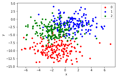
위의 scatter plot은 make_blobs function으로 생성된 dataset의 산점도이다. standard deviation 2.0으로 각 클래스 라벨은 선형으로 분리되지 않는다. 이는 딥러닝 모델이 각기 다른 결과를 충분히 낼 수 있도록 모호한 점들을 의도적으로 생성한 것이다. 결국 이러한 point는 모델의 high variance를 이끌어낼 수 있다.

MLP Model for Multi-Class Classification

생성된 dataset은 아래와 같이 설계된 모델을 통해 multi classification을 진행하게 된다.

y값을 one-hot encoding
data를 30% training data와 70% test data로 분류
15 hidden layer (with relu activation) + output layer (3 nodes with softmax)
categorical cross entropy (multi-class problem) + adam optimizer

해당 모델은 200 epoch를 돌면서 training, test data accuracy를 측정하게 된다.

# fit high variance mlp on blobs classification problem
from sklearn.datasets.samples_generator import make_blobs
from keras.utils import to_categorical
from keras.models import Sequential
from keras.layers import Dense
from matplotlib import pyplot
# generate 2d classification dataset
X, y = make_blobs(n_samples=500, centers=3, n_features=2, cluster_std=2, random_state=2)
y = to_categorical(y)
# split into train and test
n_train = int(0.3 * X.shape[0])
trainX, testX = X[:n_train, :], X[n_train:, :]
trainy, testy = y[:n_train], y[n_train:]
# define model
model = Sequential()
model.add(Dense(15, input_dim=2, activation='relu'))
model.add(Dense(3, activation='softmax'))
model.compile(loss='categorical_crossentropy', optimizer='adam', metrics=['accuracy'])
# fit model
history = model.fit(trainX, trainy, validation_data=(testX, testy), epochs=200, verbose=0)
# evaluate the model
_, train_acc = model.evaluate(trainX, trainy, verbose=0)
_, test_acc = model.evaluate(testX, testy, verbose=0)
print('Train: %.3f, Test: %.3f' % (train_acc, test_acc))
# learning curves of model accuracy
pyplot.plot(history.history['acc'], label='train')
pyplot.plot(history.history['val_acc'], label='test')
pyplot.legend()
pyplot.show()

Using TensorFlow backend.

Train: 0.833, Test: 0.774

png

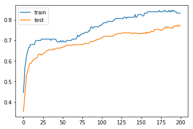
모델 결과는 84% (training data), 76% (test data)로 그래프 상으로 overfitting 되어 보이지는 않는다. 이 모델은 여러 개선 사항이 있지만 high variance를 의도적으로 적용하고 추후 model averaging ensemble과 비교하기 위해 이 상태로 둔다.

High Variance of MLP Model

의도적으로 예측시에 high variance를 가지는 모델을 구현하기 위해 위 예제 중 fit / evaulate function을 분리한다. 그 후 같은 데이터셋, 같은 모델 configuration을 가지고 반복적으로 실행한 후 변화되는 final performance를 측정한다.

주의사항
neural network은 무작위성을 사용하여 변수간의 관계를 유추하고 정답셋을 학습하도록 디자인 되었다. 따라서 같은 모델, 같은 데이터 셋을 사용하더라도 실행할 때마다 결과가 달라진다(고정된 결과값을 갖기 위한 해결책으로는 seed 값 셋팅 등이 있음). 다음의 예가 neural network에서 사용하는 무작위성 (randomness)의 일부분이다.

Randomness in Initialization, such as weights.
Randomness in Regularization, such as dropout.
Randomness in Layers, such as word embedding.
Randomness in Optimization, such as stochastic optimization.

# demonstrate high variance of mlp model on blobs classification problem
from sklearn.datasets.samples_generator import make_blobs
from keras.utils import to_categorical
from keras.models import Sequential
from keras.layers import Dense
from numpy import mean
from numpy import std
from matplotlib import pyplot

# fit and evaluate a neural net model on the dataset
def evaluate_model(trainX, trainy, testX, testy):
	# define model
	model = Sequential()
	model.add(Dense(15, input_dim=2, activation='relu'))
	model.add(Dense(3, activation='softmax'))
	model.compile(loss='categorical_crossentropy', optimizer='adam', metrics=['accuracy'])
	# fit model
	model.fit(trainX, trainy, epochs=200, verbose=0)
	# evaluate the model
	_, test_acc = model.evaluate(testX, testy, verbose=0)
	return test_acc

# generate 2d classification dataset
X, y = make_blobs(n_samples=500, centers=3, n_features=2, cluster_std=2, random_state=2)
y = to_categorical(y)
# split into train and test
n_train = int(0.3 * X.shape[0])
trainX, testX = X[:n_train, :], X[n_train:, :]
trainy, testy = y[:n_train], y[n_train:]
# repeated evaluation
n_repeats = 30
scores = list()
for _ in range(n_repeats):
	score = evaluate_model(trainX, trainy, testX, testy)
	print('> %.3f' % score)
	scores.append(score)
# summarize the distribution of scores
print('Scores Mean: %.3f, Standard Deviation: %.3f' % (mean(scores), std(scores)))
# histogram of distribution
pyplot.hist(scores, bins=10)
pyplot.show()
# boxplot of distribution
pyplot.boxplot(scores)
pyplot.show()

> 0.743
> 0.774
> 0.766
> 0.757
> 0.760
> 0.769
> 0.751
> 0.737
> 0.774
> 0.763
> 0.777
> 0.777
> 0.777
> 0.757
> 0.780
> 0.763
> 0.751
> 0.766
> 0.803
> 0.774
> 0.763
> 0.783
> 0.780
> 0.786
> 0.751
> 0.749
> 0.769
> 0.743
> 0.760
> 0.769
Scores Mean: 0.766, Standard Deviation: 0.014

png

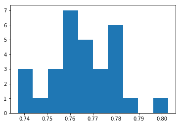
30번동안 모델을 훈련/평가하고 test data 정확도를 저장한 결과이다. 30개의 정확도 데이터가 수집되면 분포가 가우스라고 가정하고 평균 및 표준편차 관점에서 분포 점수를 산정할 수 있다. 30번에 대한 평균 결과값은 77% Accuracy, 1.4% standard deviation이다.

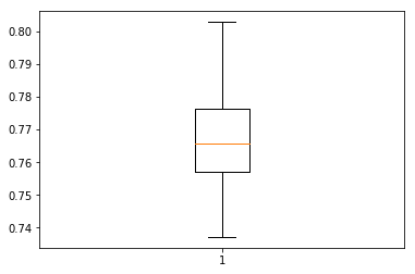
또한 가우시안 분포를 가정할 때 (histogram plot확인) 73%~81% 사이에 99% data의 존재할 것을 예상할 수 있다. (box plot의 3시그마 값) 또한 box plot의 상자값(사분위수 범위)을 확인하면 76%~78% 사이에 50%의 샘플 데이터가 존재함을 알 수 있다.

결과적으로 box plot의 73%~81%에 대한 test data의 정확도, 8% 범위는 합리적으로 variation이 높은 결과값으로 간주될 수 있다.

Model Averaging Ensemble

위와 같이 모델 error와 viariance가 높을 경우 해결 방법으로 model averaging을 사용할 수 있다. 특히, training set의 performance를 높이고 test set의 standard deviation 값을 줄이는 효과를 볼 수 있다.
이를 위해 다음과 같은 함수를 정의한다.

모델 훈련 함수 분리
앙상블 모델 멤버 리스트 취합
앙상블 결과를 이용하여 예측
앙상블 멤버의 수에 따른 테스트 정확도의 민감도 분석

# model averaging ensemble and a study of ensemble size on test accuracy
from sklearn.datasets.samples_generator import make_blobs
from keras.utils import to_categorical
from keras.models import Sequential
from keras.layers import Dense
import numpy
from numpy import array
from numpy import argmax
from sklearn.metrics import accuracy_score
from matplotlib import pyplot

# fit model on dataset
def fit_model(trainX, trainy):
	# define model
	model = Sequential()
	model.add(Dense(15, input_dim=2, activation='relu'))
	model.add(Dense(3, activation='softmax'))
	model.compile(loss='categorical_crossentropy', optimizer='adam', metrics=['accuracy'])
	# fit model
	model.fit(trainX, trainy, epochs=200, verbose=0)
	return model

# make an ensemble prediction for multi-class classification
def ensemble_predictions(members, testX):
	# make predictions
	yhats = [model.predict(testX) for model in members]
	yhats = array(yhats)
	# sum across ensemble members
	summed = numpy.sum(yhats, axis=0)
	# argmax across classes
	result = argmax(summed, axis=1)
	return result

# evaluate a specific number of members in an ensemble
def evaluate_n_members(members, n_members, testX, testy):
	# select a subset of members
	subset = members[:n_members]
	print(len(subset))
	# make prediction
	yhat = ensemble_predictions(subset, testX)
	# calculate accuracy
	return accuracy_score(testy, yhat)

# generate 2d classification dataset
X, y = make_blobs(n_samples=500, centers=3, n_features=2, cluster_std=2, random_state=2)
# split into train and test
n_train = int(0.3 * X.shape[0])
trainX, testX = X[:n_train, :], X[n_train:, :]
trainy, testy = y[:n_train], y[n_train:]
trainy = to_categorical(trainy)
# fit all models
n_members = 20
members = [fit_model(trainX, trainy) for _ in range(n_members)]
# evaluate different numbers of ensembles
scores = list()
for i in range(1, n_members+1):
	score = evaluate_n_members(members, i, testX, testy)
	print('> %.3f' % score)
	scores.append(score)
# plot score vs number of ensemble members
x_axis = [i for i in range(1, n_members+1)]
pyplot.plot(x_axis, scores)
pyplot.show()

png

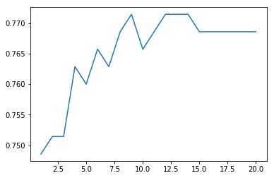
같은 training dataset을 가지고 20개의 모델을 훈련한 경우이다. 각 모델에 대한 test accuracy의 그래프를 보면 5개의 모델을 ensemble 했을 때 76% 정도로 정확도가 향상하는 것을 볼 수 있다. 5개에 model ensemble에 대한 정확도는 그 이후 모델 ensemble에 대한 평균 test data 정확도와 거의 비슷함으로 5개를 최종 ensemble model 개수로 채택한다.

마지막으로, single model 대신 5개의 모델을 ensemble 했을 때 정확도와 variance를 살펴보면 다음과 같다.

# repeated evaluation of model averaging ensemble on blobs dataset
from sklearn.datasets.samples_generator import make_blobs
from keras.utils import to_categorical
from keras.models import Sequential
from keras.layers import Dense
import numpy
from numpy import array
from numpy import argmax
from numpy import mean
from numpy import std
from sklearn.metrics import accuracy_score

# fit model on dataset
def fit_model(trainX, trainy):
	# define model
	model = Sequential()
	model.add(Dense(15, input_dim=2, activation='relu'))
	model.add(Dense(3, activation='softmax'))
	model.compile(loss='categorical_crossentropy', optimizer='adam', metrics=['accuracy'])
	# fit model
	model.fit(trainX, trainy, epochs=200, verbose=0)
	return model

# make an ensemble prediction for multi-class classification
def ensemble_predictions(members, testX):
	# make predictions
	yhats = [model.predict(testX) for model in members]
	yhats = array(yhats)
	# sum across ensemble members
	summed = numpy.sum(yhats, axis=0)
	# argmax across classes
	result = argmax(summed, axis=1)
	return result

# evaluate ensemble model
def evaluate_members(members, testX, testy):
	# make prediction
	yhat = ensemble_predictions(members, testX)
	# calculate accuracy
	return accuracy_score(testy, yhat)

# generate 2d classification dataset
X, y = make_blobs(n_samples=500, centers=3, n_features=2, cluster_std=2, random_state=2)
# split into train and test
n_train = int(0.3 * X.shape[0])
trainX, testX = X[:n_train, :], X[n_train:, :]
trainy, testy = y[:n_train], y[n_train:]
trainy = to_categorical(trainy)
# repeated evaluation
n_repeats = 30
n_members = 5
scores = list()
for _ in range(n_repeats):
	# fit all models
	members = [fit_model(trainX, trainy) for _ in range(n_members)]
	# evaluate ensemble
	score = evaluate_members(members, testX, testy)
	print('> %.3f' % score)
	scores.append(score)
# summarize the distribution of scores
print('Scores Mean: %.3f, Standard Deviation: %.3f' % (mean(scores), std(scores)))

> 0.766
> 0.757
> 0.771
> 0.774
> 0.769
> 0.780
> 0.783
> 0.763
> 0.769
> 0.760
> 0.763
> 0.769
> 0.766
> 0.769
> 0.766
> 0.780
> 0.771
> 0.760
> 0.740
> 0.771
> 0.769
> 0.769
> 0.766
> 0.771
> 0.769
> 0.771
> 0.757
> 0.774
> 0.760
> 0.780
Scores Mean: 0.768, Standard Deviation: 0.008

test dataset의 정확도는 77%로 single model일 경우와 거의 차이가 없다. 여기서 주목할 만한 점은 standard deviation 값이 single model인 경우 1.4%, 5개의 ensemble 모델인 경우 0.8%로 0.6% 정도 감소하였다는 것이다.
이것은 model의 variance를 줄임으로써 test dataset의 정확도를 높이고 신뢰성 있는 결과를 도출할 수 있음을 의미한다. 이렇게 variance 값이 낮은 모델은 높은 신뢰성을 가지고 결과적으로 final model의 average performance를 높이게 된다.

https://inspiringpeople.github.io/data%20analysis/feature_selection/

Reference

https://machinelearningmastery.com/model-averaging-ensemble-for-deep-learning-neural-networks/

YounKyung Jang

Model Averaging을 통한 Ensemble 방법

Keras에서 Model Averaging 하는 방법

Multi-Class Dataset 만들기

MLP Model for Multi-Class Classification

High Variance of MLP Model

Model Averaging Ensemble

Reference

댓글남기기

참고

Tonnetz 음악이론을 딥러닝에 접목시키기

Music21 라이브러리를 활용한 미디 데이터 분석

AI와 함께 작곡한다면?

2019년 상반기 회고 및 다짐

YounKyung Jang

Keras에서 Model Averaging 하는 방법

Multi-Class Dataset 만들기

MLP Model for Multi-Class Classification

High Variance of MLP Model

Model Averaging Ensemble

Related Post

Reference

댓글남기기

참고

Tonnetz 음악이론을 딥러닝에 접목시키기

Music21 라이브러리를 활용한 미디 데이터 분석

AI와 함께 작곡한다면?

2019년 상반기 회고 및 다짐